Diversity in Life
  • Home
  • Diversity in Life Blog
  • Software
  • diveRsity online
  • R-peer-grp

diveRsity v1.7.6 update: The problem of bootstrapping bias

1/27/2014

1 Comment

 
By Kevin Keenan

A new version of diveRsity is now available for download from 'CRAN'. It can also be downloaded using the method described here. While most of the updates in this version are minor, some are more substantial. One of these is the inclusion of an automated bias correction for confidence intervals (CIs) estimated for pairwise differentiation. Below is a coded demonstration of the problem of bias when estimating confidence intervals for diversity/differentiation statistics from bootstrapped data.

The code

Load diveRsity and calculate pairwise differentiation, including \( 95\% \) Confidence Intervals (using 1000 bootstrap iterations).

 # load diveRsity library(diveRsity)
# run fastDivPart on "Test_data" (1000 bootstraps)
data(Test_data)
system.time({
pwDiff <- fastDivPart(Test_data, pairwise = TRUE,
bs_pairwise = TRUE, WC_Fst = TRUE,
bootstrap = 1000, parallel = TRUE)
})
    user  system elapsed 
2.810 0.054 456.167

Since Test_data contains genotype data for six population samples, fastDivPart will calculate confidence intervals for 15 separate pairwise estimates of \( G_{ST} \) (Nei & Chesser, 1983), \( G^{'}_{ST} \) (Hedrick, 2005), \( D_{Jost} \) (Jost, 2008) and \( \theta \) (Weir & Cockerham, 1984). We can plot these point estimates along with CIs as follows (N.B. by setting the argument plot = TRUE in the original call, these results will be plotted automatically).

Plotting the results

 # View the pairwise results data
names(pwDiff)
 [1] "standard"     "estimate"     "pairwise"     "meanPairwise" "bs_pairwise"   

We can see that the pairwise bootstrap results are located at bs_pairwise. This object within pwDiff contains separate data tables for each of the four statistics listed above. All data tables have the same structure, so we can just look at one, \( D_{Jost} \).

 pwDiff$bs_pairwise$djostEst  
                       actual      mean    BC_mean Lower_95%CI Upper_95%CI BC_Lower_95%CI BC_Upper_95%CI
POP1_1 vs. POP2_1 0.6002342 0.5850703 0.6002342 5.169e-01 0.647625 0.5320938 0.6627891
POP1_1 vs. POP3_1 0.0006103 0.0011152 0.0006103 4.645e-06 0.003614 -0.0005003 0.0031092
POP1_1 vs. POP4_1 -0.0002870 0.0002585 -0.0002870 -7.567e-05 0.001304 -0.0006211 0.0007581
POP2_1 vs. POP3_1 0.5903311 0.5742200 0.5903311 5.086e-01 0.635704 0.5246634 0.6518151
POP2_1 vs. POP4_1 0.5933083 0.5783549 0.5933083 5.139e-01 0.641400 0.5288839 0.6563533
POP3_1 vs. POP4_1 0.0010899 0.0018571 0.0010899 3.038e-04 0.004484 -0.0004634 0.0037167

We can see that the output for each of the four statistics estimates contains seven data columns. We are interested in comparing the difference between the standard CIs and the bias corrected CIs.

 # plot using ggplot2
library(ggplot2)
# create a djost dataframe from our pwDiff results to reduce typing
djost <- as.data.frame(pwDiff$bs_pairwise$djostEst)
# The column names cause problems, so we can change them as follows:
colnames(djost) <- c("actual", "mean", "bcMean", "bucLow", "bucUp", "bcLow", "bcUp")
# plot the point estimates for each of your four pw comparisons
# with uncorrected and corrected 95% CIs
CI_type <- as.factor(c(rep("uc", nrow(djost)), rep("bc", nrow(djost))))
ggplot(djost, aes(x = c(1:nrow(djost),1:nrow(djost) + 0.5),
y = c(actual, actual), colour = CI_type)) +
geom_errorbar(aes(ymin = c(bucLow, bcLow), ymax = c(bucUp, bcUp)),
width = 0.3) +
geom_point() +
ylab(expression(D["Jost"])) +
xlab("Pairwise Comparison")

plot of chunk plt3

A figure demonstrating the difference in bias corrected and uncorrected \( 95\% CIs \) derived from 1000 bootstrap iterations. Blue lines represent the uncorrected CI, while pink lines represent the bias corrected CIs.

Of particular note is the fact that often the uncorrected CIs don't even encompass the sample estimates. This occurs as a result of the known upward bias associated with bootstrapping these types of statistics. Another important point of notes is the increased risk of type I error seen for two of the pairwise comparisons when using uncorrected CIs. In these comparisons, the uncorrected CIs do not overlap \( 0 \), suggesting differentiation between the two populations is statistically significant. However, following bias correction, these pairwise differentiation estimates are no longer significantly different from \( 0 \) (i.e. they overlap \( 0 \)).

From this example, it is clear that correcting for bias in bootstrapped differentiation estimates is important. In line with this, diveRsity now provides automatic bias correction in the fastDivPart function.

N.B. divPart does not have this capability since it is no longer supported.

References

  • Hedrick, P. (2005) A standardized genetic differentiation measure. Evolution, 59, 1633–1638

  • Jost, L. (2008) GST and its relatives do not measure differentiation. Molecular Ecology, 17, 4015–4026

  • Jost, L. (2008) GST and its relatives do not measure differentiation. Molecular Ecology, 17, 4015–4026

  • Keenan, K., McGinnity, P., Cross, T. F., Crozier, W. W., Prodöhl, P. A. (2013), diveRsity: An R package for the estimation and exploration of population genetics parameters and their associated errors. Methods in Ecology and Evolution, 4: 782–788. doi: 10.1111/2041-210X.12067

  • Weir, B. & Cockerham, C. (1984) Estimating F-statistics for the analysis of population structure. Evolution, 38, 1358–1370
1 Comment

Why use mapply?

10/17/2013

0 Comments


By Kevin Keenan

The apply family of functions in R are extremely useful. I've been using them for quite a while now, generally in place of for loops. However, they are not particulary intuative for R beginners, in the same way that loops can be.

One apply function that I have never paid much attention to in the past is mapply. I've attempted to use it a few times but could never make sense of the help file and just resorted to loops instead. This morning, however, I was trying to calculate some statistics from the independent element of two lists that I had generated, and was determined to avoid using a for loop (my default position when writing R code).

A quick google search suggested that mapply was the way to go. After some fumbling around and lots of trial and error, the scales dropped from my eyes as I held 'CTRL+ENTER' (in RStudio of course) and the stop icon dissappeared as if it was never there. Previously, when running similar calculations using for loops, the stop icon might have remained tauntingly for up to a minute, maybe more.

It appears that mapply is not only easier to use than I previously thought, but also lightening fast. Let the code below be a testament to its power:

Example code

For the purpose of illustration, imagine we have two lists of length 100,000, each element being a matrix of 100 random variables with 10 columns and 10 rows.

Imagine that we are interested in calculating the product of each matrix (i.e. \( mat1 \times mat2 \)). Let's have a look at the speed difference between using a for loop and mapply.

 # generate the data
list1 <- list()
list2 <- list()
for (i in 1:1e+05) {
list1[[i]] <- matrix(rnorm(100), ncol = 10)
list2[[i]] <- matrix(rnorm(100), ncol = 10)
}
# Calculate the matrix products using a 'for' loop
system.time({
listProd1 <- list()
for (i in 1:1e+05) {
listProd1[[i]] <- list1[[i]] * list2[[i]]
}
})
 ##    user  system elapsed 
## 32.33 1.34 34.31
   # Calculate the matrix products using 'mapply'
system.time({
listProd2 <- mapply(FUN = `*`, list1, list2, SIMPLIFY = FALSE)
})
 ##    user  system elapsed 
## 0.34 0.03 0.38
  # Test to make sure both methods do the same thing
listProd1[[1]] == listProd2[[1]]
 ##       [,1] [,2] [,3] [,4] [,5] [,6] [,7] [,8] [,9] [,10]
## [1,] TRUE TRUE TRUE TRUE TRUE TRUE TRUE TRUE TRUE TRUE
## [2,] TRUE TRUE TRUE TRUE TRUE TRUE TRUE TRUE TRUE TRUE
## [3,] TRUE TRUE TRUE TRUE TRUE TRUE TRUE TRUE TRUE TRUE
## [4,] TRUE TRUE TRUE TRUE TRUE TRUE TRUE TRUE TRUE TRUE
## [5,] TRUE TRUE TRUE TRUE TRUE TRUE TRUE TRUE TRUE TRUE
## [6,] TRUE TRUE TRUE TRUE TRUE TRUE TRUE TRUE TRUE TRUE
## [7,] TRUE TRUE TRUE TRUE TRUE TRUE TRUE TRUE TRUE TRUE
## [8,] TRUE TRUE TRUE TRUE TRUE TRUE TRUE TRUE TRUE TRUE
## [9,] TRUE TRUE TRUE TRUE TRUE TRUE TRUE TRUE TRUE TRUE
## [10,] TRUE TRUE TRUE TRUE TRUE TRUE TRUE TRUE TRUE TRUE
 listProd1[[1000]] == listProd2[[1000]]
 ##       [,1] [,2] [,3] [,4] [,5] [,6] [,7] [,8] [,9] [,10]
## [1,] TRUE TRUE TRUE TRUE TRUE TRUE TRUE TRUE TRUE TRUE
## [2,] TRUE TRUE TRUE TRUE TRUE TRUE TRUE TRUE TRUE TRUE
## [3,] TRUE TRUE TRUE TRUE TRUE TRUE TRUE TRUE TRUE TRUE
## [4,] TRUE TRUE TRUE TRUE TRUE TRUE TRUE TRUE TRUE TRUE
## [5,] TRUE TRUE TRUE TRUE TRUE TRUE TRUE TRUE TRUE TRUE
## [6,] TRUE TRUE TRUE TRUE TRUE TRUE TRUE TRUE TRUE TRUE
## [7,] TRUE TRUE TRUE TRUE TRUE TRUE TRUE TRUE TRUE TRUE
## [8,] TRUE TRUE TRUE TRUE TRUE TRUE TRUE TRUE TRUE TRUE
## [9,] TRUE TRUE TRUE TRUE TRUE TRUE TRUE TRUE TRUE TRUE
## [10,] TRUE TRUE TRUE TRUE TRUE TRUE TRUE TRUE TRUE TRUE

We can see that there is a massive (in computation terms) difference in the performance of these two methods. Although I don't know for sure, I suspect the time penalties in the for loop are due to growing the list from scratch which takes time, and is not the best way to do things.

Reproducibility

 ## R Under development (unstable) (2013-09-29 r64014)
## Platform: x86_64-w64-mingw32/x64 (64-bit)
##
## attached base packages:
## [1] stats graphics grDevices utils datasets methods base
##
## other attached packages:
## [1] knitr_1.5.1
##
## loaded via a namespace (and not attached):
## [1] digest_0.6.3 evaluate_0.4.7 formatR_0.9 stringr_0.6.2
## [5] tools_3.1.0
0 Comments

diveRsity update: v1.5.1

9/9/2013

0 Comments

 
By Kevin Keenan
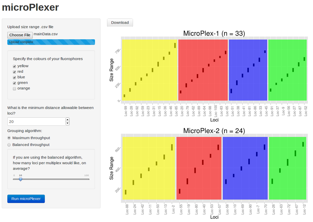
I have just submitted an update to diveRsity to CRAN. In this version you will find a handy new function, microPlexer, which launches a shiny web app, allowing you to design high-throughput microsatellite multiplexes based on locus size ranges and fluorophore technology. With the aid of ggplot2 and some modified code from Whinston Chang's excellent website, these multiplex groups can be visualised for downstream PCR tests.

The web app can also be accessed remotely at http://glimmer.rstudio.com/kkeenan/microPlexer/.

Below is an example of the multiplex plots produced by microPlexer:
Picture
0 Comments

Beware the sprintf: diveRsity v1.5.0 released

5/22/2013

0 Comments


By Kevin Keenan

Picture
To say I don't like Apple Mac would be unfair. For example, I own an iPhone, and iPod and an iPad (I know I know, that sounds very like the old canard, "I'm not X, some of my best friends are Y", but for tech geeks). The reason I've never owned a Mac computer is probably some combination of their lack of popularly among my peers, and their cost relative to PCs of similar specs.
I never thought my lack of familiarity with Mac OS X would cause me any problems though, it is based on UNIX after all. Recently however, I have been struggling with an apparent bug in the diveRsity package source code, and it quickly became clear that the users having trouble were all Mac OS X peeps. I couldn't reproduce their problem on my Windows XP, Windows 7 or Ubuntu (Linux) operating systems, so I asked a colleague to test the  problem on their Mac (thanks Deirdre!). Sadly they weren't imagining it. The problem was mine to solve. I quickly went about trying to install Mac OS X on my PC (which isn't the most straight forward process by the way), and manged to get it working using a combination of Ubuntu and virtualbox (instructions can be found here).

After installing Mac OS X I went about the hefty task of finding an ambiguous bug in just shy of 9,000 lines of poorly annotated code (I wrote most of diveRsity late at night when being meticulous was the least of my worries). I finally localised the bug to the chunk of code below:
 if (gp == 3) { 
plMake <- function(x) {
matrix(sprintf("%06g", as.numeric(x)),
nrow = nrow(x), ncol = ncol(x))
}
} else if (gp == 2) {
plMake <- function(x) {
matrix(sprintf("%04g", as.numeric(x)),
nrow = nrow(x), ncol = ncol(x))
}
}
The code basically ensures that all elements in a given matrix have the same number of characters making downstream processing with 'substr' easier. For example if one element in matrix x is 'NA', when passed to the sprintf function with the argument "%06g", it becomes '    NA'. So the sprintf function simply adds 'padding' to the character string (in this case four space/empty characters making the element a total of six character in length). Well that the way it's was supposed to work anyway.

Apparently because 'sprintf' is just a wrapper for the C-level function 'printf', the arguments "%06g" and "%04g" have undefined behaviour which is OS dependent. The above example holds true in Windows and Lunix (i.e. space/empty character padding), but in Mac OS X, the function results in 'leading zero padding' not leading spaces. This means that where the code downstream was expecting either '    NA' (four spaces and NA) or '  NA' (two spaces and NA), in Mac OS X the actual string was either '0000NA' or '00NA'.

This bug resulted in the creation of two completely new alleles at a locus (where missing data should actually be), leading to erroneous calculation of allele frequencies downstream. To solve the problem without having to modify too much code, I simply added a conditional argument to the above code. See below:
 if (gp == 3) { 
plMake <- function(x) {
out <- matrix(sprintf("%06g", as.numeric(x)),
nrow = nrow(x), ncol = ncol(x))
if (Sys.info()["sysname"] == "Darwin") {
out[out == "0000NA"] <- " NA"
}
return(out)
}
} else if (gp == 2) {
plMake <- function(x) {
out <- matrix(sprintf("%04g", as.numeric(x)),
nrow = nrow(x), ncol = ncol(x))
if (Sys.info()["sysname"] == "Darwin") {
out[out == "00NA"] <- " NA"
}
return(out)
}
}
The latest version of diveRsity (v1.5.0) contains a fix for this bug and should be available on CRAN over the next couple of days.
Thanks to Mariah Meek and Andy Jasonowicz for first bring this problem to by attention, and all of their helpful information on the problem.

I forgot to mention that a paper introduction the diveRsity package has been accepted for publication in Method in Ecology and Evolution. Users wishing to cite diveRsity in their own research should use this resource. An 'early view' copy of the manuscript can be downloaded for free from here. R users can also type 'citation("diveRsity")' into the console to see the citation information (incl. bibtex) for the package.
0 Comments

diveRsity v1.4.6 now on CRAN

4/1/2013

0 Comments

 
Picture
The newest version of diveRsity has just been uploaded to CRAN. The major change in this version is the addition of a new function 'bigDivPart' which allows the efficient calculation of diversity partitioning and differentiation statistics for very large data sets (e.g. RAD-seq derived SNP loci). This new function uses memory efficient programming to allow the analysis of data sets containing more than 100,000 loci, on most modern laptops (e.g. I tested the function on my laptop with 6Gb RAM with a data file containing 268 individuals across 9 population samples, genotyped at 55,000 loci. The entire analysis took just over 3min and my RAM usage reached a maximum of about 3.5Gb). All detail regarding function usage can be found in the updated user manual.
0 Comments

Batch processing genepop files with diveRsity.

3/31/2013

0 Comments

 
By Kevin Keenan
Picture
A few months back I was sent an email by a useR of the the diveRsity package, asking a question which involved calculating mean pairwise parameters from hundreds of separate genepop files. It was an interesting problem that I had never considered before. The more I thought about the problem, the more I realised how important this task might be in simulation based studies such as Approximate Bayesian Computation (ABC).

These tasks generally involve the simulation of hundreds, thousands or even millions of data sets, and the subsequent estimation of a range of summary statistics from each of these. Depending on the number of data sets involved, the computational effort might be massive. 

In the case of the emailer, parallelisation seemed like a fast solution to the problem, which would allow the tasked to be scaled from a desktop to a cluster environment if needs be. The below psudo-code demonstrates the use of the 'divPart' function to calculate global diversity statistics for imaginary batches of files (e.g. assume the files being analyses are separated into 10 separate folders which represent 10 separate simulation scenarios perhaps, with each folder containing 1000 genepop files), using R.
  ########################################################### 
# Running divPart on batches of genepop files in parallel #
###########################################################
# load the diveRsity package
library("diveRsity")

# specify the top level directory under which all 'simulation'
# folders are located, by setting the working directory to it.

setwd("~/simulations")

# The directory tree might look like this:

simulations
|
---- simulation-1
| |
| ---- file1.gen
| |
| ---- file2.gen
| |
| ---- file3.gen
| ---- simulation-2
| |
| ---- file1.gen
| |
| ---- file2.gen
| |
| ---- file3.gen
| ---- simulation-3
| |
| ---- file1.gen
| |
| ---- file2.gen
| |
| ---- file3.gen

# and so on. # Next we can specify the names of our simulation folders in two ways
# manually
fold_names <- paste("simulation", 1:10, sep = "-")

# automatically (when there is only a single level below the
# top directory)
fold_names <- list.dirs(full.names = TRUE, recursive = FALSE)

# Now we can determine the names of all genepop files in each folder

file_names <- lapply(fold_names, function(x){
files <- dir(path = paste(x, "/", sep = ""), pattern = "*.gen",
full.names = TRUE)
return(files) })

# file_names will be a list of length 10. Each element will contain
# the names of all .gen files within the respective simulation folder

# Before we are ready to run the main analyses, we should set up
# the parallel environment

# load the doParallel package
library("doParallel")
# set up a cluster of 10 CPUs (one for each batch of files)
cl <- makeCluster(10)
# Export the 'divPart' function to the cluster cores
clusterExport(cl, "divPart", envir = environment())

# Now we can run the main analyses

results <- parLapply(cl, file_names, function(x){
sim_res <- sapply(x, function(y){
out <- divPart(infile = y, gp = 3, WC_Fst = TRUE)
return(out$estimate[nrow(out$estimate), 4:7])
})
return(t(sim_res)) # transpose sim_res
})

# This will generate a list (of length 10), with each element containing
# a matrix of 1000 rows (1 per file) and 4 columns (1 for each diversity
# statistic
# example of output for simulation 1
G_st_est G_hed_st_est D_Jost_est Fst_WC
0.3905 0.8938 0.8256 0.4010
0.5519 0.8719 0.6986 0.6031
0.5924 0.8880 0.7092 0.6096
... ... ... ...
... ... ... ...

# these results could then be piped to further analyses or visualisation
# tools
If any of the command usage here is not clear or incorrect, please don't hesitate to contact me (either by commenting or via email). You will find my email in the diveRsity package documentation.
0 Comments

R  1 : 0 Mendeley

2/15/2013

0 Comments


By Kevin Keenan

I'm frequently reminded of the wise words spoken to me by my PhD supervisor, "Computers just do what people tell them. If something goes wrong, it's probably the humans fault". Back then it was pretty common to hear me cursing my computer for not doing what I wanted. Now I have a much better appreciation of the simplistic way computers 'think', so I know that my laptop won't draw a plot the way I want it to unless I tell it EXACTLY how I want it drawn, down to the last pixel.
Despite my advocation of the rule; 'blame yourself first and the computer second' when something goes wrong, computers still baffle me sometimes. Why did my laptop crash first thing on Monday morning? I still haven't found out.

The story goes, I logged in at about 0730, checked my emails, read a couple of paper abstracts and installed some automatic updates. I noticed that my system needed a reboot for one of the updates to take effect, so I complied. Following the restart I was greeted with an empty desktop without the Ubuntu unity launcher icons or the system menu. I could still operate the system from the terminal, but the system seemed very unstable, besides, that's no way to operate a computer with so much graphics power to spare. I went about trawling through Google searches for 'missing unity launcher', 'unity launcher and menu bar don't appear' and the like. I tried lots of the proposed solutions but nothing worked. After a full day of trying to fix the problem, and knowing that I had a looming deadline for some stuff I need a fully operational system for, I came to the decision to do a clean re-install of Ubuntu. I had been meaning to this for a while because previously I was only using the wubu version, and I had some problems with activating the hibernate function as well as my fn key functionality.

The re-install went smoothly when I finally got some disc space back from my greedy Windows 7 installation. I restored my backups and installed my preferred packages. Within a couple of hours I was back to normal with everything working beautifully, or so I thought.
I realised that I had forgotten about Mendeley, my preferred ref manager. I quickly installed it and logged in, that was when things got messy. I had stupidly forgone the option to sync my library with a cloud source, instead choosing to host my library in single directory on my Windows 7 partition. This was no problem because on the wubi installation the Ubuntu file system was just a virtual extension of the windows system, so the directory path was pretty standard. Now however this was not the case and I was greeted with thousand of broken links in mendeley, which could no longer locate the relevant PDFs :-(

All I could do was note my error and move on. I needed to re-read all of my PDF into Mendeley and regenerate my library. The problem was that I stupidly (again) asked Mendeley to organise my PDFs in a really cumbersome way. All PDFs were located in folders divided by publication/author_name/paper_name. If you can't imagine that, it basically means that for every single file (2,384) I would have to navigate through three folder levels to copy it and paste it to my new library. F**k that!

I knew there would be a nice easy Linux solution to collapse the directory tree and copy all PDFs, but I don't like easy. I also like to see just what can't be done in R. I went about creating a function to basically take a file pattern argument (e.g. .pdf, .txt, .xlsx) and look for all files containing this pattern and copy them to a single directory of my choice. Sounds simple doesn't it. It is. The breadth of capabilities that R has never cease to amaze me. I always tell people that "it is much more that just a place to do your t-tests or regressions. It's a programming language too".

The code below will basically look in the current working directory (i.e. the top level directory) for any other directories recursively. Then, for each located directory it will check if there are any of the relevant file types (i.e. those containing the specified patterns) and copy them to a directory named 'fileSort-[out]' under the working directory. The code will not make any changes to the source folders so your data is safe.
Click this link to download a source code file.

edit: Following a useful suggestion, I have include a new argument which allows the files to be written to a user-defined location on the system.

 # This function will look for all instances of files containing the pattern 
# specified in the argument 'patterns', and copy them to a single directory
# named 'fileSort-[out]' under the working directory.
# Source files are unmodified
# Written by Kevin Keenan 2013
# Feel free to use, modify and redistribute as you wish
fileSort <- function(patterns = NULL, new.location = getwd()){
  ptn <- patterns
  # Define the file copier/mover function
  cpmvFILE <- function(dirs = NULL, patterns = NULL){
    if(!is.null(dirs)){
      dirs = dirs
      patterns = patterns
      root <- getwd()
      sapply(dirs, function(x){
        names <- dir(path = x, pattern = patterns, ignore.case = TRUE)
        if(length(names) != 0 ){
          sapply(names, function(y){
            file.copy(from = paste(x, "/", y, sep = ""),
                      to = paste(new.location, "/", y, sep = ""),
                      overwrite = FALSE, recursive = FALSE)
          })
        }
      })
    }
  }
  # list the first level of directories 
  dirsIn <- list.dirs(full.names = TRUE, recursive = TRUE)
  # remove the first directory when path is given
  
  # Create a directory into which all relevent files will be written
  dir.create(new.location, sep = ""), showWarnings = FALSE)
  
  # run cpmvFILE, assigning res to x to prevent printout
  x <- cpmvFILE(dirs = dirsIn, patterns = ptn)
  # remove x
  rm(x)
} 
0 Comments

diveRsity v1.4.2 released [repost]

1/26/2013

0 Comments

 
by Kevin Keenan
This post is to announce the release of version 1.4.2 of the diveRsity package. This new version contains a new major function 'divBasic', which allows users to calculate basic population parameters such as allelic richness, HWE and heterozygosity. The basic usage of 'divBasic' is:
 divBasic(infile = NULL, outfile = NULL, gp = 3) 
Version 1.4.2 also incorporates this new function into the 'divOnline' web app. Users can download 'divBasic' results in a psudo-publication ready format using the 'divOnline' web app. To launch the web app simply type the following into the R console:
 divOnline()          # only works if diveRsity is loaded 
# or
diveRsity :: divOnline # works if diveRsity is not loaded
The new version also introduces a new argument 'pairwise' to the major function 'div.part'. This new argument allows user to skip the calculation of pairwise diversity statistics, which can be time consuming for large data sets. The general usage of the 'div.part' function is:
 div.part(infile = NULL, outfile = NULL, gp = 3, 
pairwise = FALSE, WC_Fst = FALSE,
bs_locus = FALSE, bs_pairwise = FALSE,
bootstraps = 0, Plot = FALSE, parallel = FALSE)
For a more detailed explanation of the diveRsity package and its functionality you can download a user manual here.
0 Comments

Some bugs are harder to catch than others: programming in R

1/10/2013

0 Comments

 
By Kevin Keenan
Picture
I have a piece of code which reads genepop format files containing genotypic data and calculates lots of basic parameters like allele frequencies and proportions of missing data per locus etc. I generally use this code in wrapper functions like 'div.part' from the diveRsity package to calculate these basic values for use in more complex analyses. Recently I have adapted the code to allow me to resample k samples of n individuals from a large panmictic population of m individuals in an attempt to assess the Type I error rate associated with specific statistical tests under various sampling routines. Changing the code wasn't particularly difficult and I began running the simulations this morning. However, every once in a while my code would terminate with the following error:

 Error in if(pTotal == 0){ : missing value where TRUE/FALSE needed 
Now, I'm a pretty haphazard coder so I've see this error message a million times. Usually the problem is obvious, maybe I haven't included flow control for missing data or something simple like that. This time however I could not see the problem. I spent quite a while looking through the code, double checking each relevant line of the the other function I was using which contained the line:
 if(pTotal == 0){ 
No matter how much I looked at it, I just couldn't see the problem. I finally decided to look through the results from the code which reads the genepop file to see if the problem might be here and not in the function which was actually returning the error.
It turns out that this code contained the most obscure bug I've ever seen. It would only cause a problem under the most improbable conditions for microsatellite data from 'real' populations. Basically I was using the R function 'apply' to convert columns of a matrix into tables which list the number of occurrences of each allele at a particular locus. However for some reason if all tables generated using apply are the same length (i.e. all loci have the same number of alleles), the function will simplify the results to a matrix rather than the usual list of tables. This change in results format meant that all parameters calculated from this point on were wrong. Here's the code that caused the problem:  
 afTab <- function(x){ 
apply(x, 2, table)
}
And the simple fix:
 afTab <- function(x){ 
lapply(x, function(i){
return(table(x[,i]))
})
}
In the fixed code, I can now force the function afTab to return a list of table because lapply will not simplify the results, but rather maintain the list structure required by downstream code.

Good stuff!
0 Comments

diveRsity v1.3.6 now available

1/3/2013

1 Comment

 
By Kevin Keenan
Picture
diveRsity v1.3.6 has just be submitted to CRAN. This new version now contains a function to calculate the statistical significance of genetic heterogeneity between population samples. A new function allowing users to launch diveRsity-online locally is also included.

1 Comment
<<Previous
    Tweet

    About the authors

    Kevin Keenan is currently working towards a PhD in population and evolutionary genetics.  
    His general research interests include; small scale intraspecific genetic divergence, speciation and phylogeography.

    Uncle Mick is currently reading genetics at the University of Manchester.
    His interests include; the role of non-coding RNA in regulatory processes, molecular processes associated with sequencing technology, and the interactions between genotype and phenotype.

    Categories

    All
    Analysis
    Ancient Dna
    Cell Biology
    Conservation
    Evolution
    Fish Genetics
    Northern Ireland
    Programming
    R
    Religion

    Blogroll

    R-bloggers

    Archives

    January 2014
    October 2013
    September 2013
    May 2013
    April 2013
    March 2013
    February 2013
    January 2013
    December 2012
    October 2012
    August 2012
    July 2012

    RSS Feed

Powered by Create your own unique website with customizable templates.